The Naive Shuffle Algorithm
by Daniel Dyla
Aside from saving time, why are programmers always told not to write code that has been written for us? Short answer: you don’t know what you don’t know.
Imagine you were writing an application in which you needed to shuffle a string. Instead of looking up the standard library function, you decided to implement it yourself because a shuffle is a simple piece of code and it would be quicker to write it than it would be to go to the documentation and find the right function. Besides, implementing things like this is fun right? Here is a simple shuffle algorithm.
import random

def naive(input):
    input = list(input)
    n = len(input)
    for i in range(n):
        j = random.randint(0,n-1)
        input[i], input[j] = input[j], input[i]

    return "".join(input)
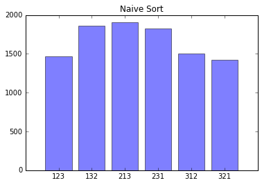
If you can already see the problem with this code then congratulations, you don’t need to read the rest of this post. This code works by iterating through the list and swapping the current element with another random element. If you are not familiar with shuffle algorithms it may be difficult to see where this code is broken. The break is so subtle that it may go years without being detected. First, let’s see what happens when we run it 10000 times.

Looking at this image, it should be clear that the shuffle function is unfairly
favoring some permutations over others. To figure out why, the easiest
explanation requires some basic math. For any string of length n, there are
n! possible permutations. In our naive shuffle algorithm, there are n^n
possible code paths. This is because at each of n elements, there are n
possible choices for which element to swap it with (including itself). For the
simple example "123" where n=3, there are 3^3 = 27 possible code paths.
With 3! = 6 different possible permutations of the array, it is clear that
each of the 6 possible shuffles cannot be equally represented by 27 code paths,
as 6 does not evenly divide 27.
The possible permutations are as follows
123 132 213 231 312 321
The possible code paths of the naive algorithms:
123
 +- 123          - swap 1 and 1 (these are positions,
 |   +- 213      - swap 2 and 1  not numbers)
 |   |   +- 312  - swap 3 and 1
 |   |   +- 231  - swap 3 and 2
 |   |   +- 213  - swap 3 and 3
 |   +- 123      - swap 2 and 2
 |   |   +- 321  - swap 3 and 1
 |   |   +- 132  - swap 3 and 2
 |   |   +- 123  - swap 3 and 3
 |   +- 132      - swap 2 and 3
 |       +- 231  - swap 3 and 1
 |       +- 123  - swap 3 and 2
 |       +- 132  - swap 3 and 3
 +- 213          - swap 1 and 2
 |   +- 123      - swap 2 and 1
 |   |   +- 321  - swap 3 and 1
 |   |   +- 132  - swap 3 and 2
 |   |   +- 123  - swap 3 and 3
 |   +- 213      - swap 2 and 2
 |   |   +- 312  - swap 3 and 1
 |   |   +- 231  - swap 3 and 2
 |   |   +- 213  - swap 3 and 3
 |   +- 231      - swap 2 and 3
 |       +- 132  - swap 3 and 1
 |       +- 213  - swap 3 and 2
 |       +- 231  - swap 3 and 3
 +- 321          - swap 1 and 3
     +- 231      - swap 2 and 1
     |   +- 132  - swap 3 and 1
     |   +- 213  - swap 3 and 2
     |   +- 231  - swap 3 and 3
     +- 321      - swap 2 and 2
     |   +- 123  - swap 3 and 1
     |   +- 312  - swap 3 and 2
     |   +- 321  - swap 3 and 3
     +- 312      - swap 2 and 3
         +- 213  - swap 3 and 1
         +- 321  - swap 3 and 2
         +- 312  - swap 3 and 3
It is easy to see that 123 is possible 4 times and 132 is possible 5 times out of the 27 code paths. Assuming a good rng (all paths are equally likely), this means 132 is more likely to be output than 123. Now let’s see the Fisher-Yates shuffle algorithm. It is almost the same as our naive algorithm, but for one simple change. As it iterates through the list, at each element it chooses a random later element (or itself) rather than just choosing a random element.
def fisheryates(input):
    input = list(input)
    l = len(input)
    for i in range(l):
        j = random.randint(i,l-1)
        input[i], input[j] = input[j], input[i]

    return "".join(input)
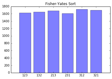
Intuitively, it would seem that this algorithm is less random. Wouldn’t it be worse to limit yourself to only swapping with later elements? Let’s test this algorithm the same way we tested our naive algorithm.

As seen in the example above, the output of this function is much more fair.
To see why this is, let’s go through the same math we did before. For the
Fisher-Yates algorithm, let’s figure out how many possible code paths there
are. At the first element, there are n possible choices (all elements in the
array), at the second element, there are n-1 possible choices (ignore all
earlier elements), continue this all the way until the last element. n *
(n-1) * (n-2) * (n-3) * ... * 2 * 1 = n!, which leaves us with n! possible
code paths. This is encouraging since it is the same number of possible
permutations, therefore it is at least possible that every output is equally
likely. This is a strong improvement over impossible. For the simple example
"123" where n=3, there are 3! = 3*2*1 = 6 possible code paths. With 3!
= 6 different possible permutations of the array, it is clear that 6 divides 6
and the algorithm is not yet proven broken as it was for the naive algorithm.
The possible permutations are as follows
123 132 213 231 312 321
The possible code paths of the Fisher-Yates algorithms:
123
 +- 123          - swap 1 and 1
 |   +- 123      - swap 2 and 2
 |   +- 132      - swap 2 and 3
 |
 +- 213          - swap 1 and 2
 |   +- 213      - swap 2 and 2
 |   +- 231      - swap 2 and 3
 |
 +- 321          - swap 1 and 3
     +- 321      - swap 2 and 2
     +- 312      - swap 2 and 3
It is easy to see that every possible output shows up once and is therefore (assuming a good rng) equally likely.
Download the code as a Jupyter notebook here.
Subscribe via RSS
